Microsoft Excel is a powerful data management tool that helps us analyze and interpret data in Data Science.
When it comes to formatting data, Excel has a wide range of techniques to enhance the worksheet’s appearance. In this article, you will learn different ways to transpose Excel data.
What Is Excel Transpose?
In Excel, Transpose is used to switch the orientation of an array. It converts the vertical range to a horizontal range or vice versa, helping us sort unformatted data into the correct order. In this write-up, you will learn three different techniques that you can use to transpose data in Excel.

How to Transpose in Excel (Best Three Approaches)
Transposing Excel data can be tricky. Follow the methods below, along with a detailed step-to-step guide, in order to transpose data effortlessly.
Paste Special Transpose
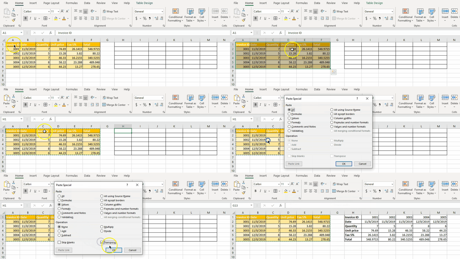
- Step 1: First, select the range that you want to transpose.
- Step 2: You will find the Copy option on the Home tab in the Excel ribbon or right-clicking the entire range.
- Step 3: Next, select a new location where you want to paste the transposed data.
- Step 4: Click on Paste Special. Find this option by navigating to the Home tab → Clipboard section → Paste → Paste Special. This option is also available when you right-click on the cell where you want to paste.
- Step 5: Then the Paste Special dialog box appears. Now, click on Values (to paste only values) and select the Transpose option on the bottom right. This step is the most crucial as we want the data to be transposed.
- Step 6: Click on OK.
The transposed data is successfully pasted to the new location.

The Paste Special feature in Excel allows you to control the formatting of the content that is being pasted. This feature can be used to copy the original content and paste the transposed data.
Look at the demo and follow the steps below to understand how to use the "Paste Special" option to transpose data.
Now, let's move forward and understand Excel's in-built TRANSPOSE function.
TRANSPOSE Excel Function
As the name suggests, the TRANSPOSE Excel function can be used to transpose data in Excel.
The syntax is:
|
=TRANSPOSE(array) |
Here, the array stands for a range of cells to be transposed.
Watch the demo displayed below to get a better understanding of how to use the TRANSPOSE function.

Follow these simple steps:
- Select the range of cells where you want the output transposed data.
- TRANSPOSE is an array formula; hence you need to select the exact number of cells.
- Suppose, if your table's range is 5x6, i.e., 5 rows and 6 columns, you must select 6x5 range, i.e., 6 rows and 5 columns, for the transposed data.
- Now, enter the formula =TRANSPOSE(A1:F5)
- Don't press Enter! You need to execute array formulas by pressing Ctrl+Shift+Enter.
- Note: Transpose is an array formula. An array formula must be entered by pressing a key combination of Ctrl+Shift+Enter so that the formula bar puts a set of braces around the formula.
- This is done to tell Excel that the output will be an array of data and not a single cell.
- The data will now be transposed.
Transpose Table Without Zeros
The Excel Transpose function converts the blank cells into zeros. In order to copy the same blank values while transposing, you need to use the IF function along with TRANSPOSE.

The procedure is similar to using the Excel Transpose function. Except here, we use the formula as:
=TRANSPOSE(IF(A1:F5="","",A1:F5)).
The IF function checks if the value is blank. If yes, it returns an empty string to transpose.
Finally, let's learn how to transpose data using the Power Query Tool.
Using Power Query Tool
Power Query is the most powerful data automation tool found in Excel 2010 and its later years.
Power Query is available as a free add-on in Excel 2010 and 2013, which you can download from Microsoft's website. It is a built-in tool starting with Excel 2016 and is available in the Get & Transforms Data Section under Data Tab.
Transposing your dataset with the help of Power Query is simple and can be done by following the steps below:
- First, select the range of data that you want to transpose.
- Go to the Data tab → Get & Transform Data section → From Table/Range and click on it. This will open the Power Query Editor.

- On the editor, go to the Transform tab → Table section → Use First Row as Headers → Use Headers as First Row. By selecting this option, all the headers (Invoice ID, Date, Unit Price, Tax, and Total) move to the first row.

- Now, click on the Transpose option, which is available in the same section. This will transpose the data.

- Select the option- ‘Use First Row as Headers’. This will ensure that the first row of transposed data is a header.

- Finally, click on the File tab → Close & Load.

The transposed data will now be loaded to a new Excel sheet.

This is what ‘how to transpose Excel data’ is all about.
Conclusion
This article has covered the different techniques that you can take to transpose Excel data. Manually transposing data can be very time-consuming. Hence, we hope this article has given you a deeper insight into various approaches that can be taken.
If you have any queries concerning the article, feel free to mention it in the comments section, and our experts will get back to you at the earliest.
You can also go the extra mile and enhance your Excel skills by enrolling in the Data Science Bootcamp offered by Simplilearn.
