
Often in Data analytics, there arises a necessity of comparing multiple columns to find the differences that could be decisive for reporting. Doing this manually could take hours and days based on the dataset you're working with. What if there is a way to fix this in a fraction of seconds?
What Do You Mean by Comparing Columns in Excel?
Comparing columns in Excel is a simple act of checking each cell in Excel against the target cells to identify a match, and in case the match is missing, then display a relevant message.
With the basics discussed, you can move ahead with the practical part.
Become a Data Science Expert & Get Your Dream Job
Caltech Post Graduate Program in Data ScienceExplore ProgramHow to Compare Two Columns in Excel?
- Make sure the entire dataset is selected.
- Click on the Home tab.
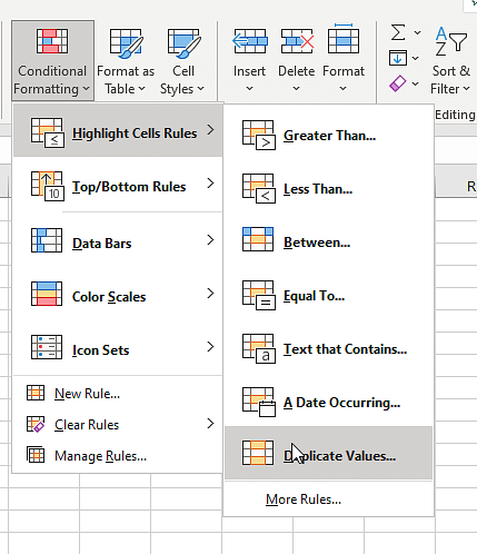
- Select 'Conditional Formatting' from the Styles group.
- Select Highlight Cell Rules by hovering your cursor over it.
- In the Duplicate Values section, click the button.
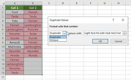
- Make sure that 'Duplicate' is selected in the Duplicate Values dialogue box.
You will execute column data comparison of the following sample data.

You must try the three different ways to compare columns in Excel, as mentioned below.
- Conditional Formatting in Excel
- Using Equals Operator
- Using LookUp Function
Conditional Formatting in Excel
Conditional Formatting in Excel is one of the simplest ways to compare columns in Excel. You can execute it in simple steps, as shown below.
Step 1
Select all cells in the spreadsheet

Step 2
Conditional Formatting
Navigate to the "Home" option and select duplicate values in the toolbar. Next, navigate to Conditional Formatting in Excel Option.
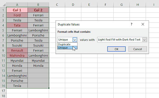
A new window will appear on the screen with options to select "Duplicate" and "Unique" values. You can compare the two columns with matching values or unique values.
Duplicate Values
Unique Values
With the first type of column comparison understood, you will move to the next type by implementing the equals operator.
Your Career as a Data Scientist is Waiting!
Caltech Post Graduate Program in Data ScienceExplore ProgramUsing Equals Operator
Another simple way to compare columns in Excel is by using the equals operator. You can execute it with the following steps.
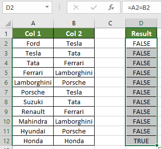
Create a new result column and add the formula for individual cell comparison, as shown below.
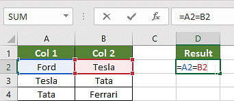
Excel will deliver the result as FALSE for every unsuccessful comparison and TRUE for every successful comparison, as shown below.
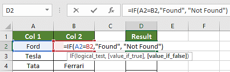
You can make minor tweaks to the formula to deliver customized messages using the "IF" clause with custom messages for "TRUE" and "FALSE" values, as shown below.
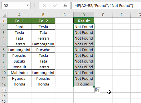
The final result will be displayed as follows.
Moving ahead, you will try using the VLookUp Function in Excel to compare columns in Excel.
Join one of the hottest industries today and upgrade your salary with Simplilearn’s Caltech Post Graduate Program In Data Science. Enroll today!
Using LookUp Function
Follow the detailed steps discussed below to use the VLookUp Function to compare individual cells.
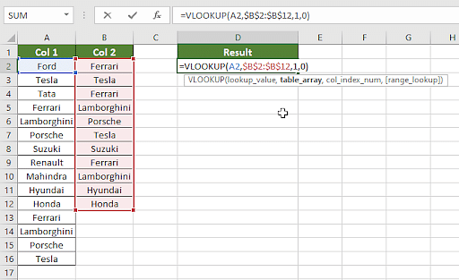
Create a new result column and add the VLookUp Formula to compare individual cells, as shown below.
Start your Dream Career with the Best Resources!
Caltech Post Graduate Program in Data ScienceExplore ProgramYou can drag the formula to all the cells to obtain the desired result, as shown below.
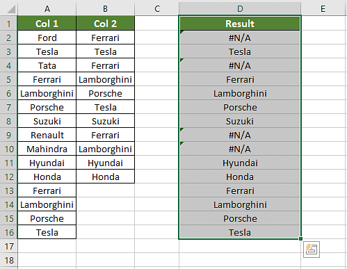
You can see traces of failed comparisons displayed as errors. You can modify your formula using the "IFERROR" clause to avoid such errors, as shown below.
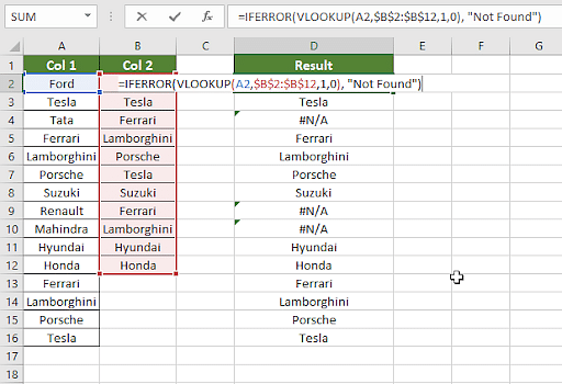
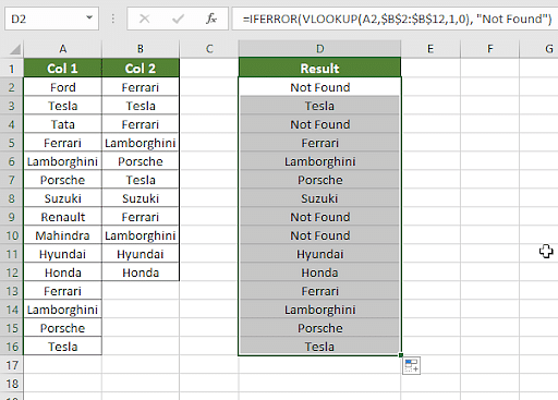
Now, you can copy-paste or drag the modified formula to all the cells to get the final error-free result, as shown below.
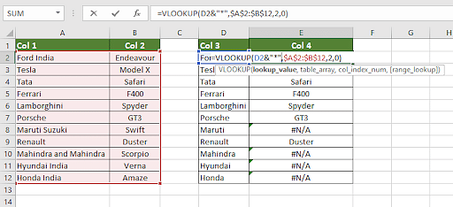
Unlike the sample data, the real-world scenarios might vary a little. For example, the comparison between the two individual cells might end up "FALSE" even if both the cells represent the same data. Now, take a better look at it with the help of the image below.
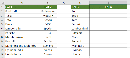
The data in columns 1 and column 3 are the same. But, there is an additional extension to a few cells.
Example: Ford India in the first cell of column 1 and Ford in the first cell of column 3.
The standard VLookUp might end up delivering "FASLE" as a result. You can use wildcards as a minor tweak to the data to avoid this, as shown below.
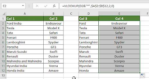
Now, drag the modified formula cell to all the cells, and the resultant data will be shown as follows.
With that, you can conclude this tutorial on Compare columns in Excel.
Become a Data Scientist by learning from the best with Simplilearn’s Caltech Post Graduate Program In Data Science. Enroll Now!
Next Steps
You have learned how to compare columns in Excel. Pivot Charts in Excel can be your next learning endeavor as they are building blocks of data analytics with interactive dashboards in excel.
You can also check out the beginner's guide to Microsoft Excel to get more insights.
Curious about learning business analytics and data science and landing the right job? Simplilearn's Data Science course has got you covered. This Caltech Post Graduate Program in Data Science offered by Simplilearn teaches you the fundamental concepts of data analysis and statistics to help you achieve reliable decision-making. This training guides you with Power BI and delves into the statistical topics, which will help you devise data from available data to present your reports using professional-level dashboards.
Should you have any doubts, do let us know in the comments below, and our Excel experts will help you as soon as possible.